Simple Spatio-Temporal Windowing With Kafka Streams

The Big Idea

When I read about the new Kafka Streams component being developed by the Apache Kafka team, I was quite intrigued. Kafka Streams is a lightweight streaming layer built directly into Kafka. In line with the Kafka philosophy, it “turns the database inside out” which allows streaming applications to achieve similar scaling and robustness guarantees as those provided by Kafka itself without deploying another orchestration and execution layer.

Kafka gives us data (and compute) distribution and performance based on a distributed log model. Kafka Streams exposes a compute model that is based on keys and temporal windows. It works on both event streams (KStream) and update streams (KTable).

I want to work with spatial data instead of pure <key, value> data. In this post, I’ll show the simplest version of that: aggregating data into hexbins based on location and time.

The idea of hexbins are simple: create a hexagonal tiling of the space of interest and handle all the points within each hexagon together.

Hexbins are useful for visualizing density and hot spots in two-dimensional data. Overlayed on a map, hexbins can give us useful, albeit simple, insights into the geospatial distribution of some activity.

The Sample Application

To show spatio-temporal windowing in action, we’re going to build an application that determines tweet density by hour for various regions of San Francisco. All the code for this application is available on GitHub at https://github.com/tomfaulhaber/geo-window.

The application pipeline is laid out as follows with the three separate parts connected by Kafka topics:

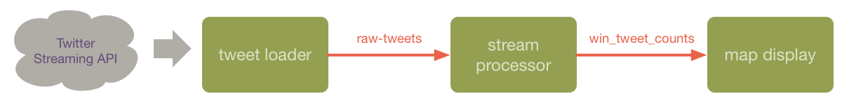
In this post, I’ll focus exclusively on the Kafka Streams portion of the pipeline. The tweet loading is done by a Clojure program here and the mapping is done in R with the code here.

I will present the application in Java. If you prefer, you can check out this version in Clojure.

The raw-tweets topic that feeds the Kafka Streams application is simply a stream of JSON-formatted tweets. This have been filtered by the geographic region around San Francisco, but this doesn’t mean that they have geographic coordinates or that those coordinates are actually in San Francisco.

Finding the hexbin

The first thing to think about is assigning each tweet to a specific hexbin. To this, we use some code translated from the D3 library, which you can find here:

1
2
3
4
5
6
7
8
9
10
11
12
13
14
15
16
17
18
19
20
21
22
23
24
25
26
27
28
29
30
31
32
33
34
35
36

public class Hexbin {
    private static final double thirdPi = Math.PI/3.0;

    private double dx;
    private double dy;

    public Hexbin(double radius) {
        this.dx = 2 * radius * Math.sin(thirdPi);
        this.dy = 1.5 * radius;
    }

    public double[] bin(double x, double y) {
        double py = y/dy;
        double pj = Math.round(py);
        double px = x/dx - ( (int)pj & 1) / 2.0;
        double pi = Math.round(px);
        double py1 = py - pj;

        if (3*Math.abs(py1) > 1) {
            double px1 = px - pi;
            double pi2 = pi + (px < pi ? -1 : 1) / 2.0;
            double pj2 = pj + (py < pj ? -1 : 1);
            double px2 = px - pi2;
            double py2 = py - pj2;

            if (px1*px1 + py1*py1 > px2*px2 + py2*py2) {
                pi = pi2 + ( ( (int)pj & 1) != 0 ? 1 : -1) / 2.0;
                pj = pj2;
            }
        }
        return new double[] {
                (pi + ( (int)pj & 1) / 2.0) * dx,
                pj * dy
        };
    }
}

The hexbinning operation is parameterized by the radius of the hexagons. In this sample we’ll use ¼ of a minute of arc.

The bin function effectively projects each x,y point onto the center of the hexagon to which it belongs. We can use this location as the spatial window key since it will be the same for all points within that hexagonal window.

Processing the input

The samples provided with Kafka Streams use the Jackson library for serializing and deserializing JSON data. Unfortunately, raw-tweets can have bad JSON data or empty messages which causes the Jackson library to throw exceptions. To deal with this, we’ll use a small wrapper class called JsonWithEmptyDeser that simply deserializes to null in that case.

I won’t reproduce that here. Curious readers can find it in the code.

Stream processing

The heart of our program is setting up and running the Kafka Streams job that will aggregate the tweets by the spatio-temporal windows.

The job is itself a pipeline of stages, like so:

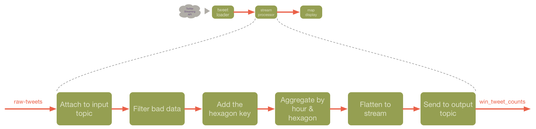
All of the connections between the stages are KStream instances except for the output of the aggregation stage which is a KTable.

You can think of a KStream as a stateless event transformer. It takes messages in from the input and transforms them onto it’s output (they can have state injected, but that’s beyond the scope of this article).

KTable on the other hand represents stateful transformations. KTable objects maintain their last emitted value for each key they have seen and emit a new value based on the old value and the new event they see. In the case of countByKey, which we use here, that value is simply an integer value that is incremented each time we see a given key. Thus, the output of a KTable operation can be seen as the sequence of updates, where an output <k,v> conceptually replaces any previous output with key = k.

The main program has four parts:

1. Set up serializer/deserializer (SerDe) objects for the job stages.
2. Define a Properties object that sets the parameters for the job.
3. Construct the stream graph.
4. Execute the stream.

Let’s walk through the code and discuss it.

Initialize the serdes

1
2
3
4
5
6
7

final Serializer<JsonNode> jsonSerializer = new JsonSerializer();
final Deserializer<JsonNode> jsonDeserializer
                = new JsonWithEmptyDeser();
final Serde<JsonNode> jsonSerde
                = Serdes.serdeFrom(jsonSerializer, jsonDeserializer);
final Serde<String> stringSerde = Serdes.String();
final Serde<Long> longSerde = Serdes.Long();

Since data traveling in and out of pipeline stages is in Kafka topics, we need to define serdes for the different datatypes we’re using. To keep things simple here, I’m only using three type: the JSON input type, strings, and longs. The only wrinkle is that we use the special wrapped JSON deserializer that I mentioned above.

Set the properties for this run

1
2
3
4
5
6
7
8
9
10
11
12
13

final String serial_number = Long.toString((new Date()).getTime());

Properties streamsConfiguration = new Properties();
// Give the Streams application a unique name.  The name must be unique in the Kafka cluster
// against which the application is run.
streamsConfiguration.put(StreamsConfig.APPLICATION_ID_CONFIG, "tweet-count-java-" + serial_number);
// Where to find Kafka broker(s).
streamsConfiguration.put(StreamsConfig.BOOTSTRAP_SERVERS_CONFIG, "localhost:9092");
// Where to find the corresponding ZooKeeper ensemble.
streamsConfiguration.put(StreamsConfig.ZOOKEEPER_CONNECT_CONFIG, "localhost:2181");
// Specify default (de)serializers for record keys and for record values.
streamsConfiguration.put(StreamsConfig.KEY_SERDE_CLASS_CONFIG, Serdes.String().getClass().getName()); streamsConfiguration.put(StreamsConfig.TIMESTAMP_EXTRACTOR_CLASS_CONFIG, TweetTimestampExtractor.class);
streamsConfiguration.put(ConsumerConfig.AUTO_OFFSET_RESET_CONFIG, "earliest");

I’ve done a few thing here that are specific to the demo/development environment.

• Each run of the application has a completely unique application name. This causes Kafka and Kafka Streams to ignore any previous application state. Usually, you’ll want applications to pick up where they left off, but in development it’s nice to be able to reload everything. See the github repo for some scripts to help with this workflow.
• The offset is set to earliest which causes the application to read the raw-tweets topic from the first message. Sometimes applications might use this in production, but usually you’re going to process just new values being added to a topic.
• I’ve hard-wired the cluster location to localhost. In a real application, this location would be injected through configuration, command line arguments, or environment variables.

We also set the timestamp extractor class. This tells Kafka Streams how to get the timestamp for each event to be used in the windowing logic. In this case, the TweetTimestampExtractor class fishes into the parsed JSON to retrieve the timestamp_ms that Twitter includes in the incoming event.

Constructing the pipeline

1
2
3
4
5
6
7
8
9
10
11
12
13
14
15
16
17
18
19
20
21
22
23
24

Hexbin hexbin = new Hexbin(1.0/240.0);
KStreamBuilder builder = new KStreamBuilder();

// The beginning of the stream pipeline is the raw JSON tweets being loaded from Twitter
KStream<String,JsonNode> tweets = builder.stream(stringSerde, jsonSerde, topicIn);

tweets
    // 1. Filter out any messages that failed to parse or have no location
    .filterNot((k,v) -> v == null || v.get("geo").isNull())
    // 2. Add the (lon,lat) of the center of the hexagon as the new key
    .map((k,v) -> {
        JsonNode coords = v.get("geo").get("coordinates");
        double[] bin = hexbin.bin(coords.get(1).doubleValue(),
                                  coords.get(0).doubleValue());
        return KeyValue.pair(String.format("%f %f", bin[0], bin[1]), v);
    })
    // 3. Count by the hour & hexagon, using Kafka Streams built-in time
    //    windowing
    .countByKey(TimeWindows.of("tweet-window", 60*60*1000), stringSerde)
    // 4. Convert the KTable back to a stream with a flattened key that can
    //    be consumed as text
    .toStream((k, v) -> String.format("%d %s", k.window().start(), k.key()))
    // 5. Send the stream to the output topic
    .to(stringSerde, longSerde, topicOut);

Building the pipeline starts with a KStreamBuilder instance, which we use to make the stream which attaches to the input topic.

We chain a succession of stream and table operations together into a single pipeline. This kind of simple progression will be very familiar to those who’ve used functional data processing environments such as Apache Spark.

The operations are, in sequence:

1. filterNot - As we’ve mentioned not all the data coming in is good. This is probably due to bugs in my twitter consumer, but real world environments often have problems like this. In this case, we look for data that’s bad or just uninteresting to us and filter it out.
2. map - The map step adds a key which is a string consisting of the longitude and latitude of the center of the hexagon that contains the location of this tweet. We can use this key as an id for the hexagon and all tweets in that hexagon will share the same key.
3. countByKey - Take the stream of input tweets and count how many are in each hexagon. As mentioned above, the step creates a KTable which maintains the previous count and emits a sequence of <k, new count> items.
4. toStream - This is really a reformatting step that flattens the time windowed key into the string “timestamp longitude latitude”. This is specific to the demo - see below.
5. to - This operation sends the output to a named Kafka topic, win_tweet_counts here, to be consumed by some other part of our ecosystem.

There are some simplifications here because this is a demo. The biggest of these is that we simply generate the change log from the end of the pipeline and let the consumer deal with that.

In a production application, the final step would usually involve pushing the data to a database, perhaps using Kafka Connect, or directly to some system (like a real-time dashboard) that just keeps the last value for keys it’s interested in.

For data sized as in the demo (which is only about 40,000 messages after filtering), it’s easy for the R code to use the dplyr library to simply take the last value for each key. We’ve constructed the key as a string such that when we use kafka-console-consumer to read the data, we get space separated lines that look like “timestamp longitude latitude count” which are easy for programs like R to read.

Running the job

1
2
3
4

KafkaStreams run = new KafkaStreams(builder, streamsConfiguration);
run.start();
Thread.sleep(50000);
run.close();

Once the stream is configured, just create a KafkaStreams object and call start on it.

Since this is a demo app, we let the stream run for 50 seconds and then stop it. This is plenty of time for the pipeline to process all the data in our sample. In production, we’d typically just have the stream running forever.

Once the job has run, I use kafka-console-consumer to put the output in a file like this:

1
2
3
4
5
6
7
8

$ ./bin/kafka-console-consumer --zookeeper localhost:2181 \
                               --topic win_tweet_counts \
                               --formatter kafka.tools.DefaultMessageFormatter \
                               --property key.deserializer=org.apache.kafka.common.serialization.StringDeserializer \
                               --property value.deserializer=org.apache.kafka.common.serialization.LongDeserializer \                              --property print.key=true \
                               --from-beginning \
                               --timeout-ms 2000 \
                               > /tmp/counts

Now, my R code can read the data from /tmp/counts

The results of the sample application

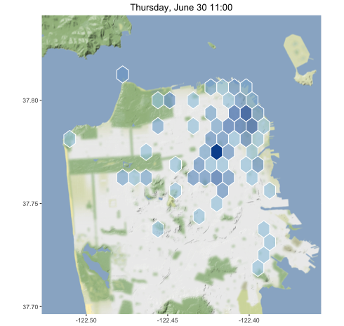
I collected geo-tagged tweets in San Francisco from June 30 to July 4, 2016, to look for interesting patterns.

Animated over the entire time period, here are the the results:

We can see some interesting patterns in this data.

On weekdays, tweets tend to be concentrated in the Market St. corridor.

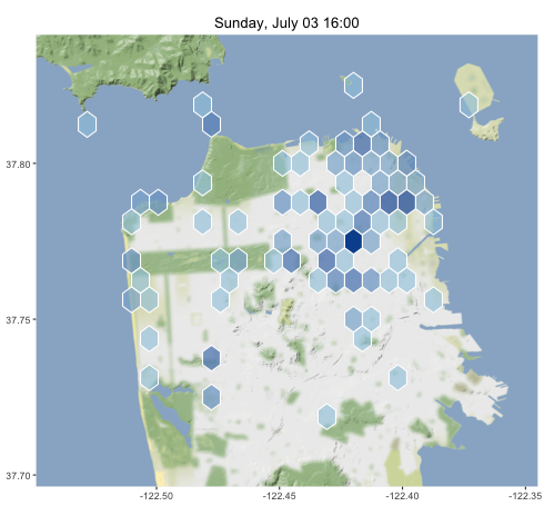
On Sunday afternoon, the tweets were spread all over the city, especially in neighborhoods like the Mission where the techies live and around Golden Gate Park and the beach.

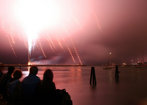
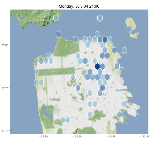
July 4th is a special day in San Francisco, when we all gather to watch the fireworks shoot up into the fog and make it glow. This is what it looks like, for those of you who haven’t had this experience:

• Stephen D./Yelp

As expected, the tweets that night were clustered along the waterfront where the fireworks were launched.

This sample is not very much data, but the exact same code should be able scale to the full twitter firehose if we launched a big enough Kafka cluster.

Limitations

Handling geospatial data at scale is a vast problem domain. Problems like the one we’ve worked on here are at the very simplest end of the scale.

I’d like to discuss some of the things that make this example limited, both to keep readers from thinking that this is more than it is and to suggest productive further work that could make these ideas much more interesting.

It’s not generalizable

The Kafka Streams code we’ve written for this application is single-purpose. If we want to make a change as small as changing the radius of the hexbin, we need to modify our program and launch a new application.

Hexbins are a limited abstraction

In addition, hexbins themselves are a very brittle abstraction for dealing with spatial data. As long as all the data we want to work with at the same time is in the same bin (as in the simple counting example that I presented above), this works well. However, most interesting spatial applications will have cases where they need to cross the hexagonal boundaries for at least some operations.

Consider finding the nearest neighbor for the different locations. In the illustration below, you can see that A’s nearest neighbor is B, which is in the same hexagon, but C’s nearest neighbor is D which is in another hexagon.

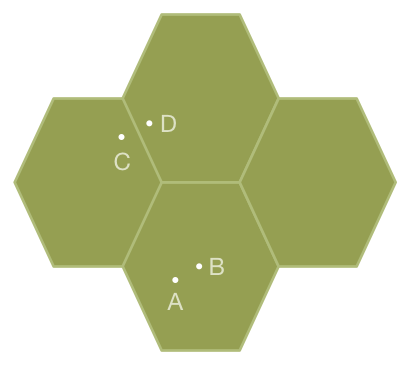
In key-value model with unordered keys like Kafka, the next hexagon might as well be infinitely far away.

Another issue with the hexbins (or any other fixed size partitioning) is that they don’t account for differences in data density in different spatial regions. A quick look at the U.S. at night from space shows us the differences in population density from place to place.

• NASA Earth Observatory/NOAA NGDC

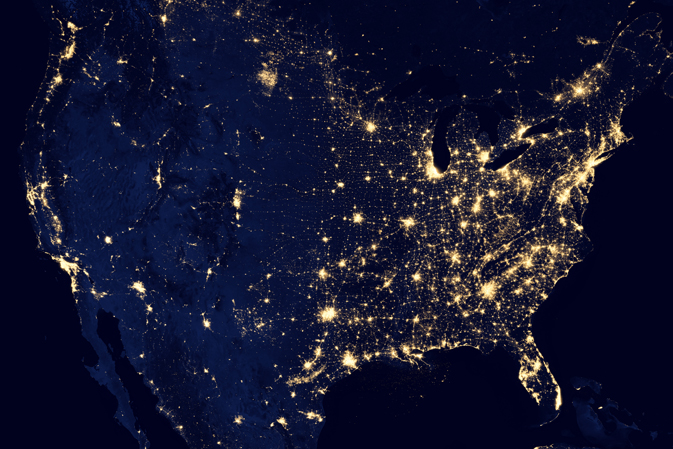
New York City and Kansas have vastly different population densities, so we certainly expect them to have vastly different data densities when measuring things that depend on human activity.

• Times Square by Divya Thakur. Kansas by Bhall87/Wikipedia.

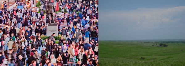
If we choose a small radius for our hexbins, we’ll end up with many empty or near-empty bins. However, if we choose a large radius, the hexbin won’t provide much discrimination in dense areas.

It’s not geographically accurate

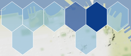
When we work in degrees, we don’t have constant area in different parts of the globe. We can see that effect here where the hexagons are squished sideways because longitude is “narrower” than latitude everywhere other than the equator.

Longitude and latitude can also present challenges of consistency since measurement can use different standards for mapping the spherical coordinate system onto oblate shape of the earth such as WGS-84.

Local regions can have their own coordinate systems as well (e.g., the Dutch RD system used for locating places in the Netherlands).

More generally, the issues of accurate determination of geospatial location are a complex subject unto themselves that I won’t discuss further here.

There’s more to the world than points

Tweets come from point locations but there are many other geospatial operations that work on more complex objects. Examples of other shapes include lines (the route of a car), polygons (the outline of a city), and radial areas (within 100 meters of an object).

Shapes can cross the hexagon boundaries which presents the challenges noted above.

Ideas for the future

In the discussion above, I use hexbins as a strawman. Hexbins are great for a certain class of problem, but not very good at some others. When I got excited about the spatial potential inherent in Kafka Streams, I was already thinking about some more advanced ideas.

There are three things that feel like good next steps:

1. Build around a data structure that’s more adaptive to density like quadtrees, PH-Trees, or space filling curves. There’s some work that’s required to match structures like these to the <key, value> model used by Kafka Streams.
2. Develop a mechanism for combining data across cells for interesting operations such as search in polygon, dynamic gridding, and nearest neighbor.
3. Make an abstraction library that lets us write applications that use these mechanisms flexibly, without rewriting the whole stream every time.

Right now this is a back burner project for me, so progess will depend on how much time I get to work on it. When I make do interesting progress, I’ll post updates here.